Geospatial workflows in Houdini
Premise
What follows is nothing more than a bunch of CLI commands and scripts that - put together - resemble a workflow useful when exploring and visualizing geospatial data.
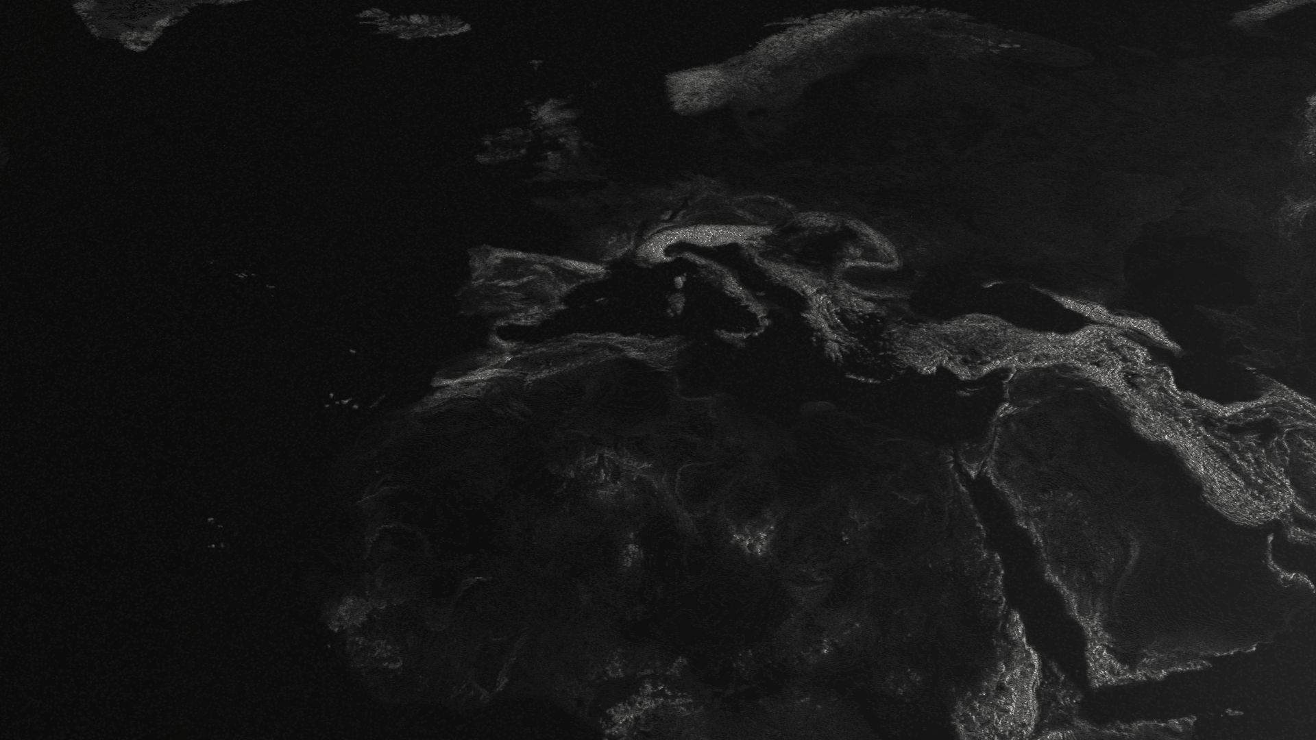
Source GeoTIFF, downsampled to 16bit
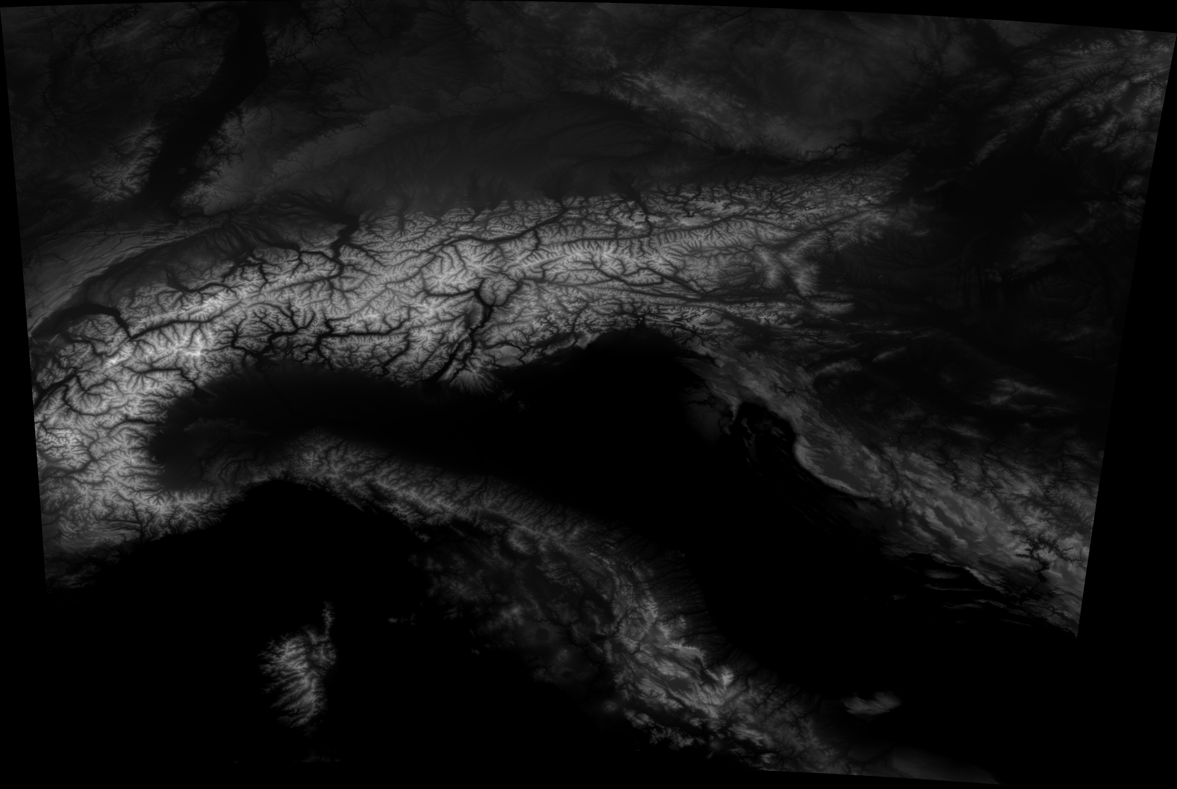
DEM data rendered in Houdini
Where to get the data?
If you're in Europe, the ESA offers open access to the DEM data captured by the Copernicus satellite. Here's the Copernicus Website: https://land.copernicus.eu/imagery-in-situ/eu-dem/
Prerequisites:
- Basic terminal/shell usage 🦞
- Some degree of familiarity with conda (or other virtual env systems)
- Beginner knowledge of Python 🐍
If you want to read more about the GDAL API for reading raster images, have a look here: https://automating-gis-processes.github.io/2016/Lesson7-read-raster.html
First of all, we need a safe way to install all the open source packages that we'll use.
My way of dealing with this kind of python projects is to encapsulate all of the data into a conda environment, so that I can keep track of the dependencies in a neat way and I avoid messing with the system python. To know more about conda and how to install it, start here: https://docs.conda.io/en/latest/
Here, we create and activate a new python 3 virtualenv:
$ conda create -n my-geospatial-env python=3
$ conda activate my-geospatial-env
Now that we have a virtualenv, let's install some useful tools of the trade:
$ conda install pip # For installing other pip-only packages
$ conda install gdal # To access the gdal* utilities
$ conda install numpy
$ pip install ipython
$ pip install notebook
$ pip install matplotlib
Converting the Coordinate Reference System of a GeoTIFF
I won't go long describing the intricacies of what is a Spatial Reference System (because I'm not a geoscientist ). Some initial knowledge can be acquired here. An awesome xkcd strip can be seen here: https://xkcd.com/977/ .
For our purposes, let's just assume that most of the times, we'll want to convert our source image into a more common CRS, which is generally WGS84, which is also how we're used to represent the earth (since it's what Google Maps uses).
The source CRS should be clearly defined in the metadata of the image or should be written in the source website.
In our case, it's EPSG:3035 (ETRS89, LAEA). Generally, there's no need to specify the input srs since gdalwarp will automatically read it for you.
$ gdalwarp mygeotiff.TIF mygeotiff_wgs84.tif -t_srs "+proj=longlat +ellps=WGS84"Then, we can create another copy of the GeoTIFF at a lower resolution, so that we can keep on working on a laptop without going crazy. Even if you're on a proper workstation with plently of RAM, you might still want to avoid working directly on a 40k x 40k image. :)
In this case, I'm setting the width to be 4000 pixels (the other dimension will follow accordingly to the source aspect ratio) :
$ gdalwarp -ts 4000 0 mygeotiff.TIF mygeotiff_wgs84_4k.tif -t_srs "+proj=longlat +ellps=WGS84"If you inspect the generated image using gdalinfo mygeotiff_wgs84_4k.tif, you'll notice that the generated image has a different aspect ratio. The source was 4k x 4k, while the new one is 4k x 2682. This shift in dimensions was generated by the CRS conversion.
The gdal suit offers also ways to generate .xyz files from our beloved GeoTIFF:
$ gdal_translate -a_srs EPSG:3035 -ot Float32 -of XYZ mygeotiff.TIF mygeotiff_wgs84.xyzHowever, doing such processing with gdal_translate usually takes a long time on my laptop, so I generally avoid this approach and go the numpy route.
Accessing the DEM data with numpy
Numpy is a general purpose library for numerical computing, which to me sounds as "don't be (too) afraid of implementing the math".
I have played around with numpy from time to time and I've always like their API and what it enables. Implementing an algorithm in numpy generally feels quite straightforward, especially if you compare its interface to the less programmer-friendly ones offered by Matlab (or even octave).
Plus, if you do things the "numpy way™" you benefit from vectorisation, which basically means that most of the computations over you dataset can run in parallel.
Here's a simple snippet showing you how to access the DEM raw values of a GeoTIFF, in just 5 lines:
>>> from osgeo import gdal
>>> dem_file_path = '/Users/vvzen/Downloads/dem/europe-copernicus/mygeotiff_wgs84.TIF'
>>> raster = gdal.Open(dem_file_path)
>>> import numpy as np
>>> raster_array = raster.ReadAsArray() # This might take a while
>>> raster_array.shape
(2682, 4000)
>>> raster.RasterXSize, raster.RasterYSize
(2682, 4000)
Now, let's leverage numpy to scatter some points over our 2D image so that we can use a lower number of points to describe our 2682x4000 image. The benefit of randomly sampling our image, especially for artistic purposes, is that reading all of the values would mean storing something like 2'682 * 4'000 = 10'728'000 points. This isn't a huge deal, but now let's consider working with the 40k x 40k image that we originally downloaded.
If you do the math, you'll end up with: 40'000 x 26'820 = 1'072'800'000 . That's a 💩 ton of data!
You we'll never ever be able to read it inside Houdini (unless you're on one of the new Mac Pros with 1.5 TBs of RAM 🙃 )
I've made a commented Notebook in order to make it extremely easy to follow along and visualize all of the steps of our processing.
In this simple example, we'll write a .ply ourselves, containing all of the x,y,z data. This way, we'll be able to later import it into houdini and triangulate it if needed.
Generating a Ply file
If you want to clone the ipython-notebook, here's the full url: https://github.com/vvzen/Houdini-Geospatial-Tools/blob/main/src/notebooks/Save_GeoTIFF_as_ply.ipynb
Use Houdini's attribfrommap
Another approach is to just load a lower quality png image (that we'll also generate using numpy + matplotlib) in Houdini.
For the sake of brevity, here's a snippet:
import os

from osgeo import gdal
import numpy as np
import matplotlib.image
import matplotlib.pyplot as plt

dem_file_path = os.path.join(os.getcwd(), "eu_dem_v11_E40N20_wgs84.tif")
dem_raster = gdal.Open(dem_file_path)
dem_raster.GetDescription()

# Luckily, GDAL offers a way to access
# the raw pixel data as a numpy array
dem_as_array = dem_raster.ReadAsArray()

# Save to disk as a lower quality 16bit png
matplotlib.image.imsave(
    "eu_dem_v11_E40N20_wgs84.png",
    dem_as_array.astype(np.float16),
    cmap="gray"
)
Then, we can load the image in Houdini using an attribfrommap node:
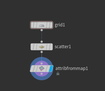
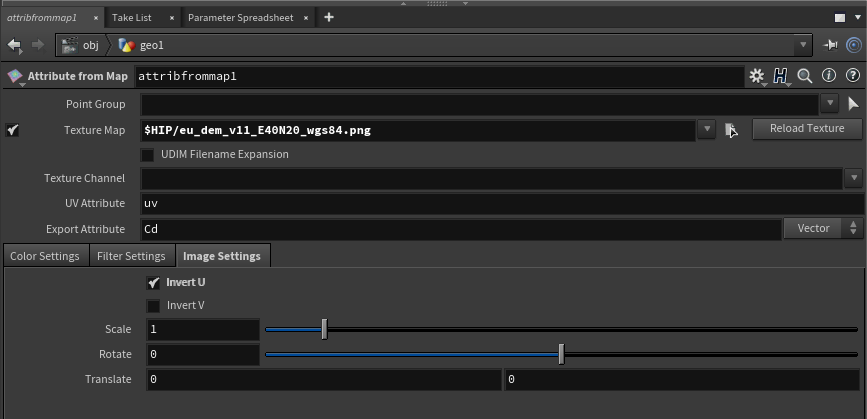
Pick whatever you like!
Personally, I like to have the dem data saved in a dummy format like .ply because it's very easy to access or parse programmatically - it's also nice to know that you can easily load that data later.
Happy geo-hacking!
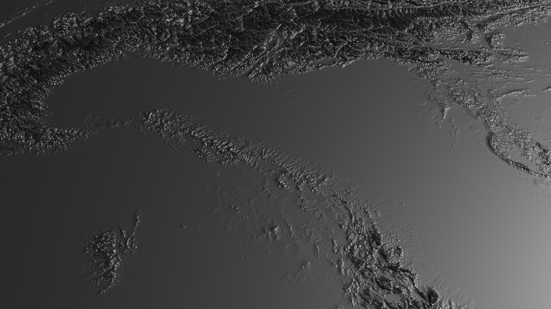
Another elevation map of Europe rendered in Houdini